The Bertrand Paradox

What does it mean for something to be randomly selected? This may at first seem like a bit of a silly question, but in fact, has deep mathematical significance. The Bertrand paradox, a seemingly simple question about triangles and circles, has driven such questions for over a century, with new work still being produced. Here I’ll take a look at the problem and run some simulations and visualizations in Python.

The problem is as follows. Suppose that we have an equilateral triangle inscribed in a circle and select a chord of the circle at random. What is the probability that the chord is longer than the triangle’s side length?

For the sake of clarity, we can easily draw the setup in Python. We’ll be doing this a few times, so I’m going to create some functions for future use. First, functions to convert from polar coordinates and calculate distance:

from math import cos, sin, pi, sqrt

def polar(r, theta):
    x = r*cos(theta)
    y = r*sin(theta)
    return (x, y)

def d(p1, p2):
    d = (p1[0] - p2[0])**2 + (p1[1] - p2[1])**2
    return sqrt(d)

and two functions for some help with plotting:

import matplotlib.pyplot as plt
%matplotlib inline

def plot_line(p1, p2, **kwargs):
    linewidth = kwargs.get('linewidth', None)
    zorder = kwargs.get('zorder', None)
    color = kwargs.get('color', None)
    
    plt.plot(*zip(p1, p2), color = color, 
              zorder = zorder, linewidth = linewidth)

def pad(pad, r):
    upper = r + pad
    lower = -upper
    plt.xlim(lower, upper)
    plt.ylim(lower, upper)

and finally our function to plot our triangle and circle and store some values we’ll need later:

from itertools import combinations

def setup(r):
    plt.figure(figsize=(10,10))
    
    #draw circle
    circle = plt.Circle((0, 0), r, color='black', fill=False, linewidth=5)
    plt.gca().add_artist(circle)
    
    #draw triangle
    top   = polar(r, pi/2)
    right = polar(r, pi/2-(2*pi)/3)
    left  = polar(r, pi/2+(2*pi)/3)
    
    for combo in combinations([top, right, left], 2):
        plot_line(*combo, 
                  color = 'blue', 
                  zorder=10, 
                  linewidth=5)
        
    side_len = d(top, right)
    
    return top, side_len, r

So when we run:

top, side_len, r = setup(r = 1)
pad(.5, r)
plt.show()

we plot this circle with a radius of 1 and an inscribed triangle:

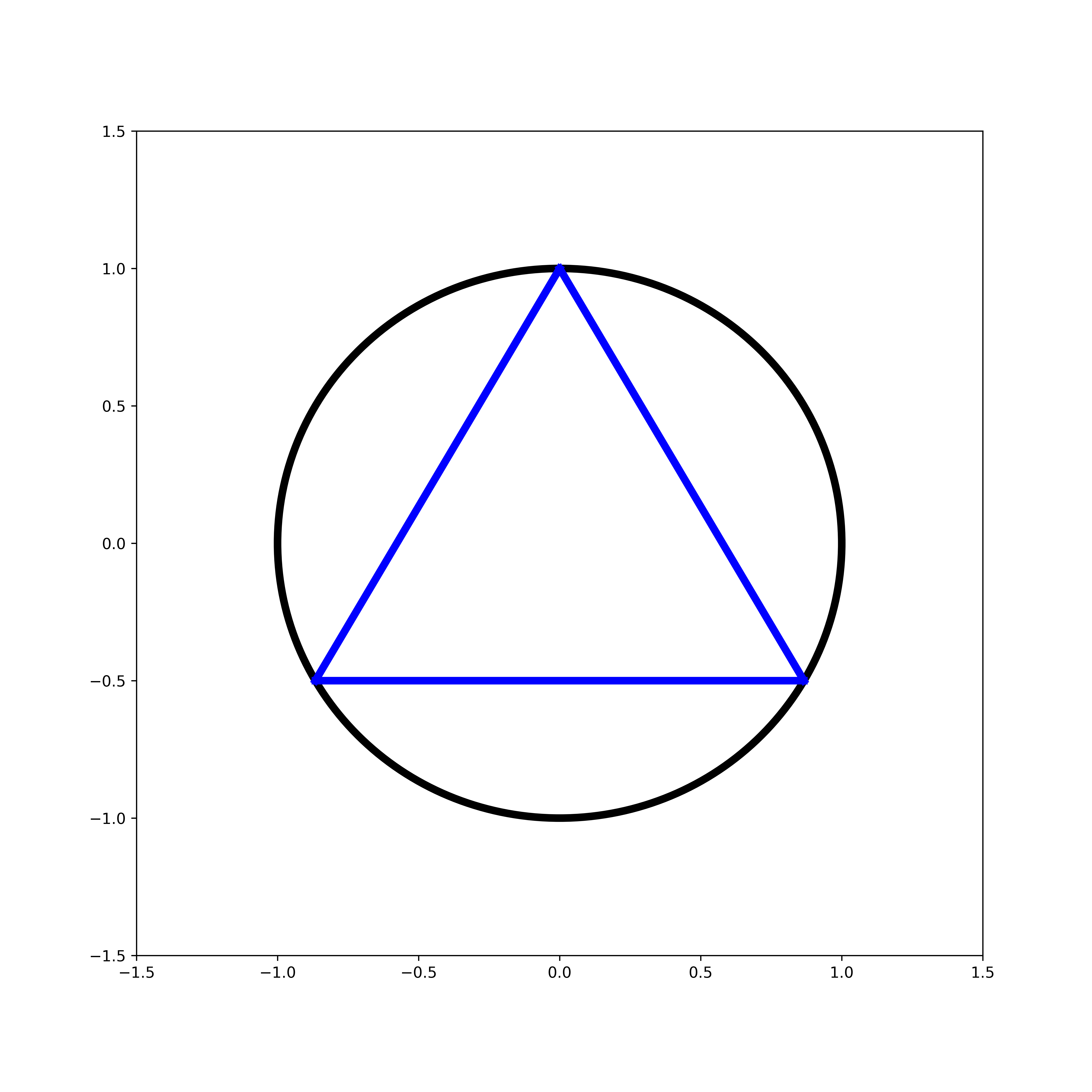
Now we need to come up with a method of selecting our random chords. We’ll take a look at three different methods.

Method 1 - Random Endpoints

For the first method, I will select two random points on the circumference of the circle and draw a cord between them. Without any loss of generality, we can rotate the chords to make our calculations and presentation a bit cleaner.
I’ll implement this in Python by using a uniform distribution to select an angle, and since we can rotate the cords, I will draw them so they all connect to the top vertex of our triangle.

from random import uniform, seed, random

top, side_len, r = setup(r = 1)

seed(10)
trial_n = 100

for i in range(trial_n):
    point = polar(r, uniform(0, 2*pi))
    if d(point, top) > side_len:
        color = 'red' 
    else:
        color = 'green'
    plot_line(top, point, color = color)
    
pad(.5, r)
plt.show()

(I have set a seed just for the purposes of saving an image.) To visualize our results I have colored any chord that is longer than our side lengths red, selecting 100 random chords:

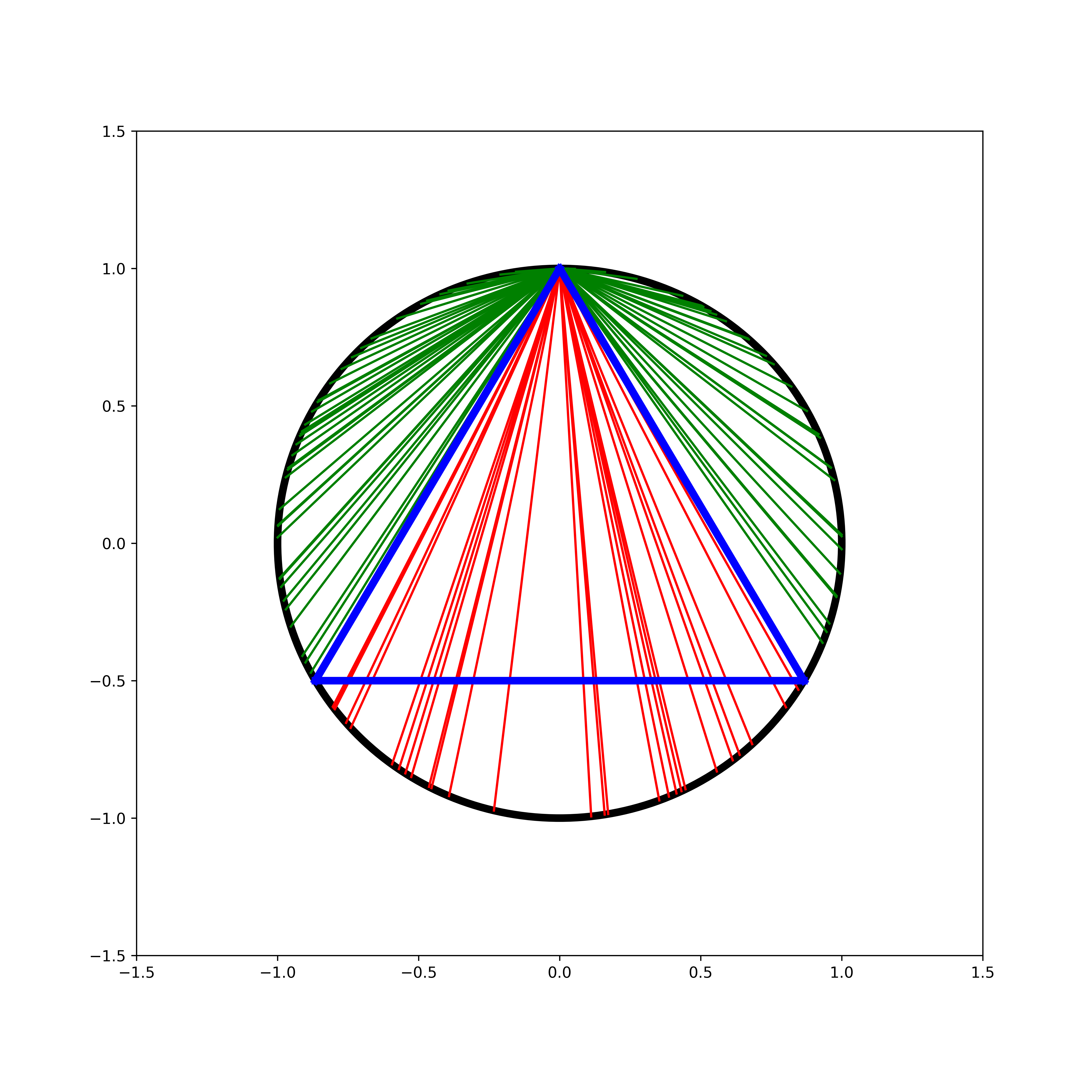
As we can see with this geometric visualization, the probability that a chord is longer than our side length approaches \(\frac{1}{3}\) as our number of trials increases. As we’ll soon see, however, this isn’t the end of the story!

Method 2 - Random Points on a Radius

Let’s try a different method of selecting our random chord. Again, I will fix an orientation by considering the radius that this perpendicular to the bottom side of our triangle:

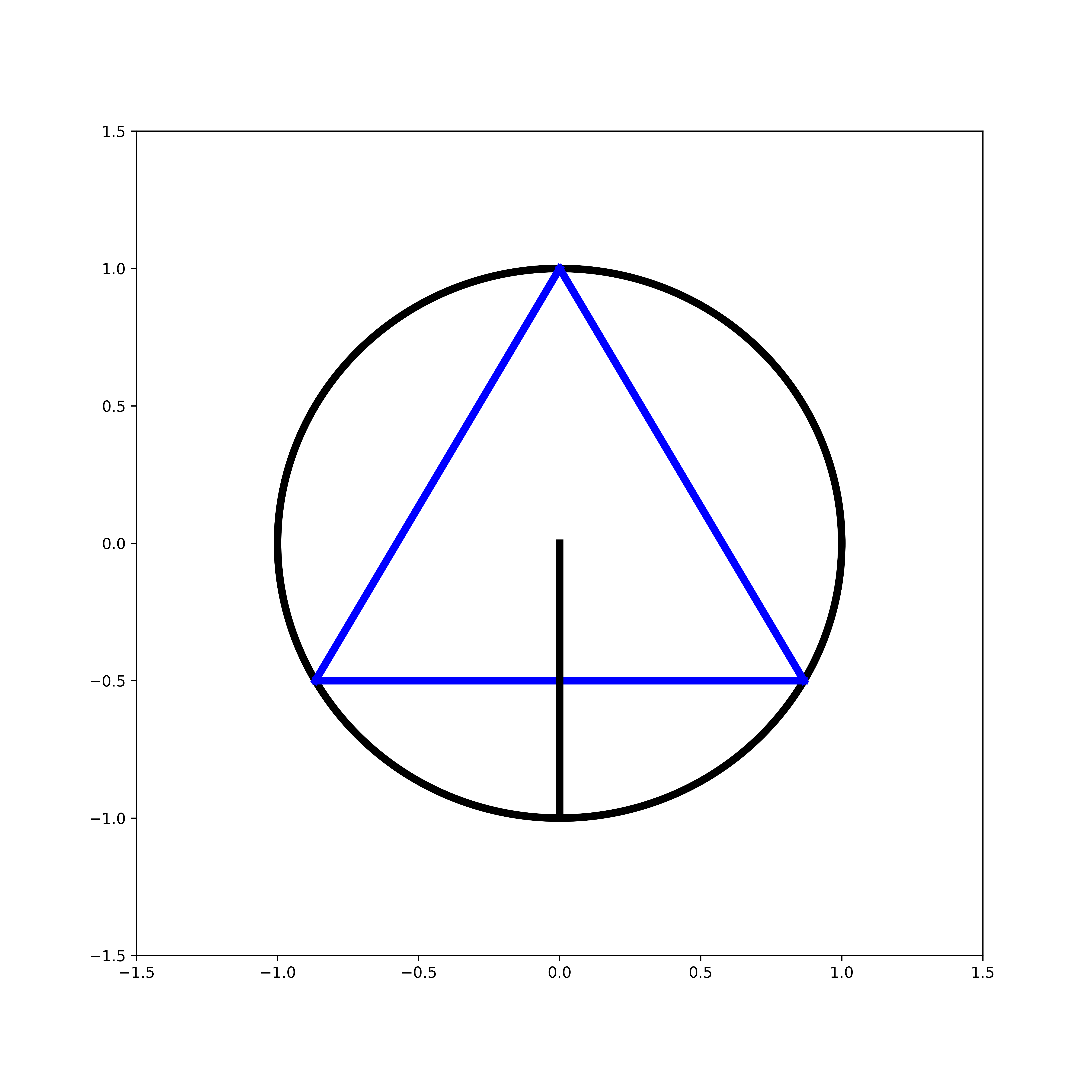
To select my chords, I will select a random point on this radius which will be the midpoint of our chord.

top, side_len, r = setup(r = 1)

bottom = polar(r, -pi/2)
plot_line(bottom, (0, 0), color = 'black', zorder=10, linewidth=5)

seed(10)
trial_n = 50

for i in range(trial_n):
    midpoint = -uniform(0, r)
    
    h = r+midpoint
    c = sqrt((r-h/2)*(8*h))
    p1 = (-c/2, midpoint) 
    p2 = ( c/2, midpoint)
    
    if d(p1, p2) > side_len:
        color = 'red' 
    else:
        color = 'green'
    
    plot_line(p1, p2, color = color, zorder=0)
    
#limits and plot
pad(.5, r)
plt.show()

The chord’s length \(c\) follows from the Intersecting chords theorem which for any chord:

gives us that: \[ c = \sqrt{8h\left(R - \frac{h}{2}\right)} \]

The simulation gives the following result:

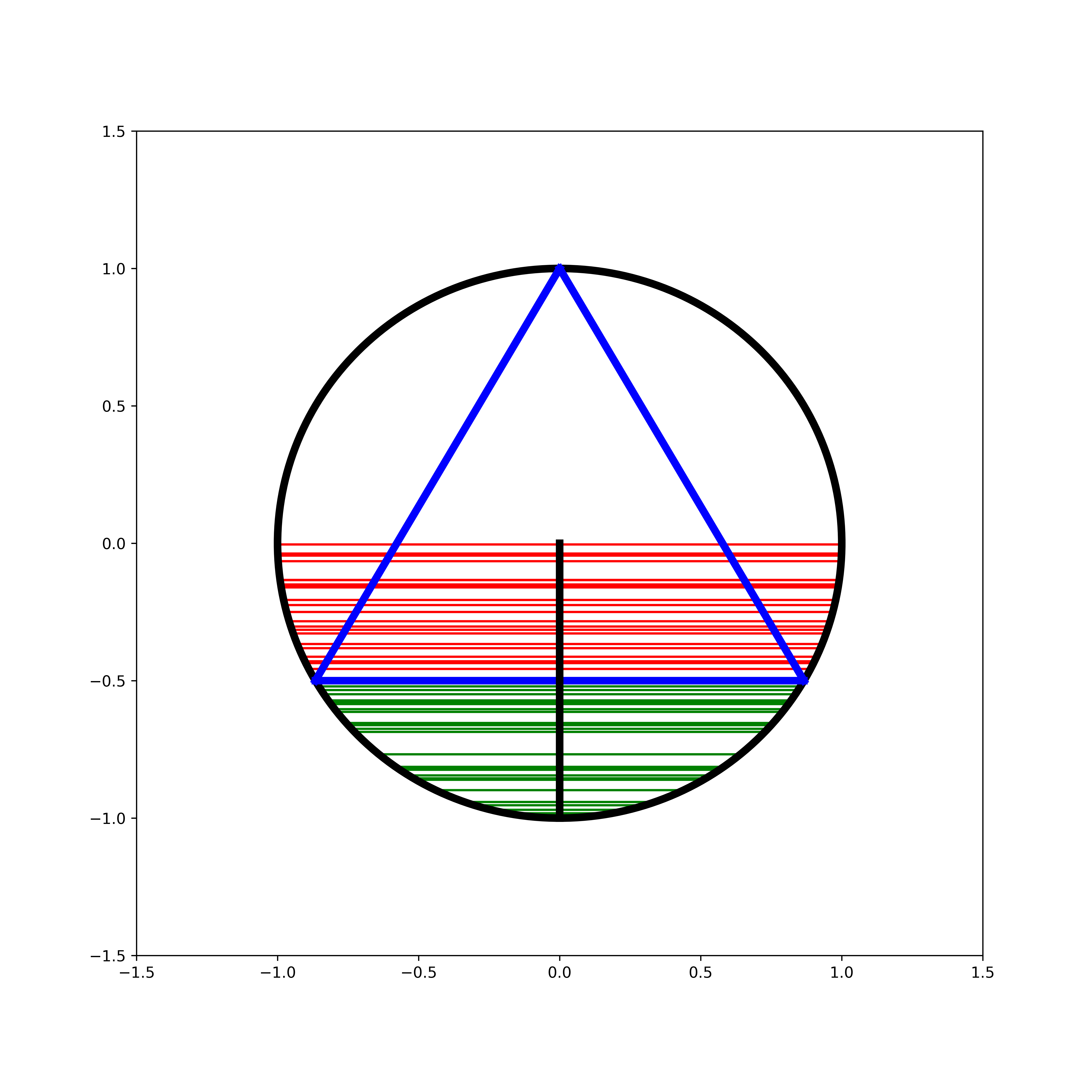
and we can see that the probability of a cord longer than the triangle’s sides is \(\frac{1}{2}\). How is this a different probability?! Let’s look at one more method before discussing.

Method 3 - Random Midpoints

For the final method, we will pick a random point within the circle, which will become the midpoint of our randomly selected chord.

This construction requires a little bit more explanation of how we actually find such a chord. Suppose that we have our randomly selected point \((x, y)\). Below I have drawn this, with the chord in blue and a line from the circle’s origin to the point in black.

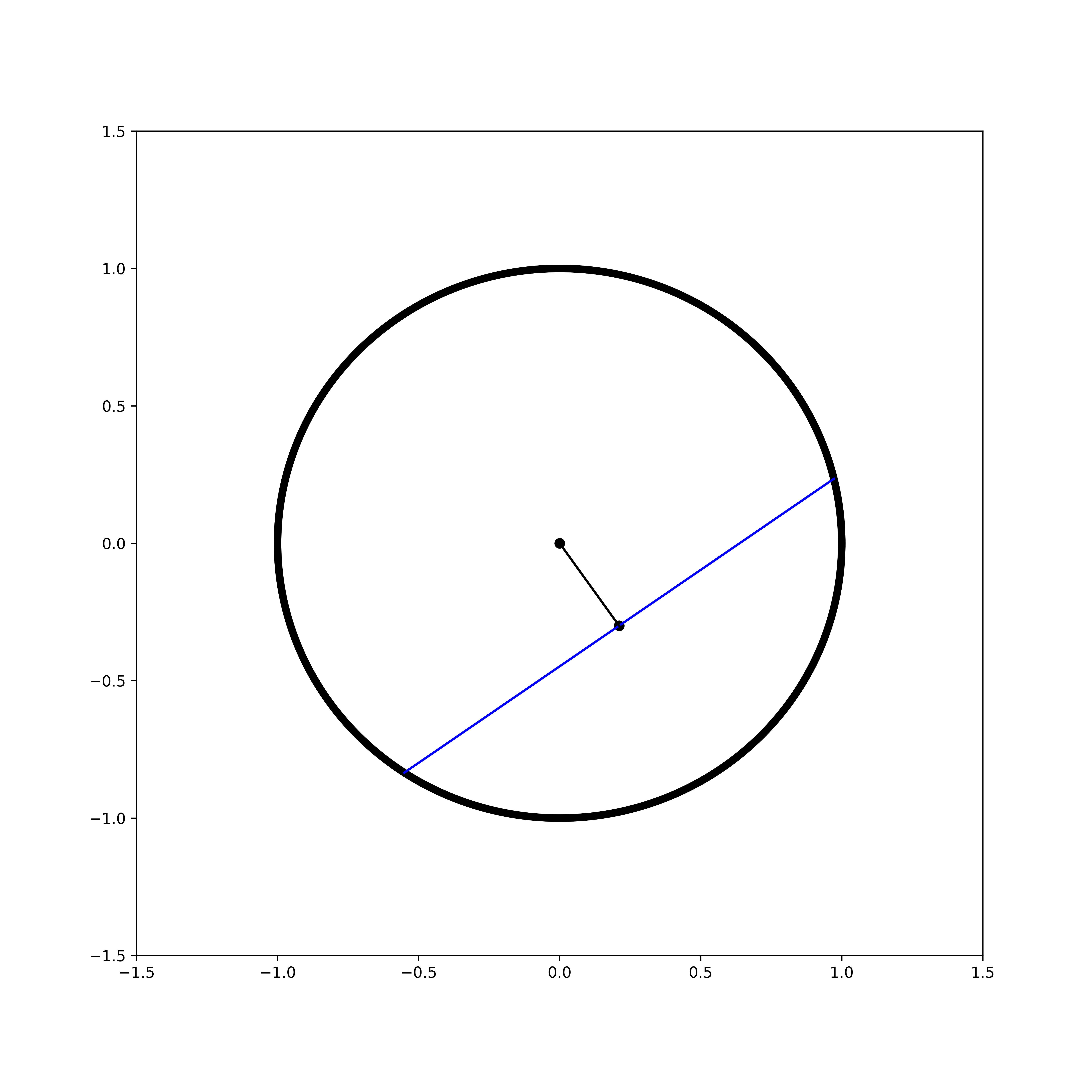
As this point is a midpoint, the line from the origin is a perpendicular bisector (see this theorem) So if we denote the origin as \((0,0)\), the slope of the chord is \(-\frac{x}{y}\), which I will denote as \(m\). I can draw the below:

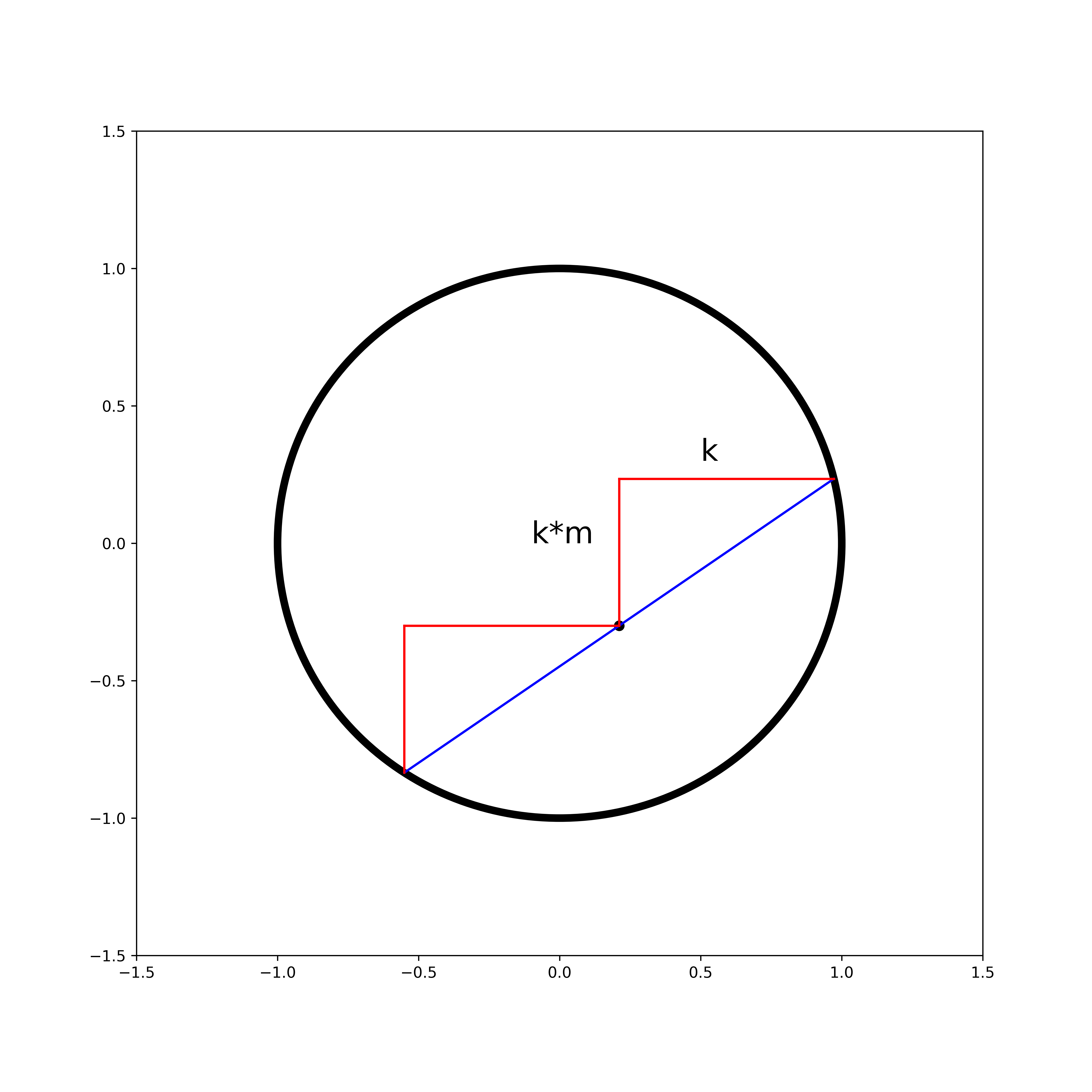
where \(k\) is some unknown real number. So the endpoints of the chord are \((x+k, y+km)\) and \((x-k, y-km)\). We can compute the distance between these and equate it to our earlier chord formula:

\[\begin{align} c^2 &= d((x+k, y+km), (x-k, y-km))^2\\ &= ((y+km)-(y-km))^2 + ((x+k)-(x-k))^2\\ &= (2km)^2 + (2k)^2\\ &= 4k^2m^2+4k^2\\ &= 4k^2(m^2+1) \end{align}\]

and solving for k gives:

\[\begin{align} k &= \sqrt{\frac{c^2}{4(m^2+1)}}\\ &= \sqrt{\frac{8h\left(R - \frac{h}{2}\right)}{4(m^2+1)}}\\ &= \sqrt{\frac{2h\left(R - \frac{h}{2}\right)}{\frac{x^2}{y^2}+1}}\\ \end{align}\]

We also must take note of how to uniformly sample points within our circle. Let our circle’s radius be denoted \(R\). If we sample uniformly for \(r\in [0, R]\) and \(\theta \in [0, 2\pi)\) we will actually end up with a distibution that is more dense in the center. We need to make our probability density function proportional by some constant \(k\) to the radius. Solving for k:

\[\begin{align} 1 &= \int_0^R f(r) \mathop{}\!\mathrm{d}r\\ &= \int_0^R kr \mathop{}\!\mathrm{d}r\\ &= \left( \frac{k}{2} r^2 \right)\bigg\vert_{r=0}^{r=R}\\ &= \frac{kR}{2} \end{align}\]

gives us \(k=\frac{2}{R}\), so that the cumulative distribution function is:

\[ \int \frac{2}{R}r \mathop{}\!\mathrm{d}r = \frac{r^2}{R} \]

taking the inverse, we see that we should sample \(\theta \in [0, 2\pi)\) and \(r\in R\sqrt{U(0, 1)}\) (Take a look at this Stack Overflow answer for another good explanation)

appropriately modifying our script:

top, side_len, r = setup(r = 1)

circle1 = plt.Circle((0, 0), r/2, color='black', fill=False, linewidth=5)
plt.gcf().gca().add_artist(circle1)

seed(10)
trial_n = 100

for i in range(trial_n):
    point = polar(r*sqrt(random()), 2*pi*random()) 
    x, y = point[0], point[1]
    
    slope = -x/y
    
    h = r-d((0, 0), point)
    c = sqrt((r-h/2)*(8*h))
    k = sqrt((c**2)/(4*slope**2+4))
    
    if c > side_len:
        color = 'red' 
    else:
        color = 'green'
    
    plot_line((x-k, y-k*slope), (x+k, y+k*slope), color = color)
    plt.scatter(*point, color = color)
    
#limits and plot
pad(.5, r)
plt.show()

and then seeing the results of our simulation:

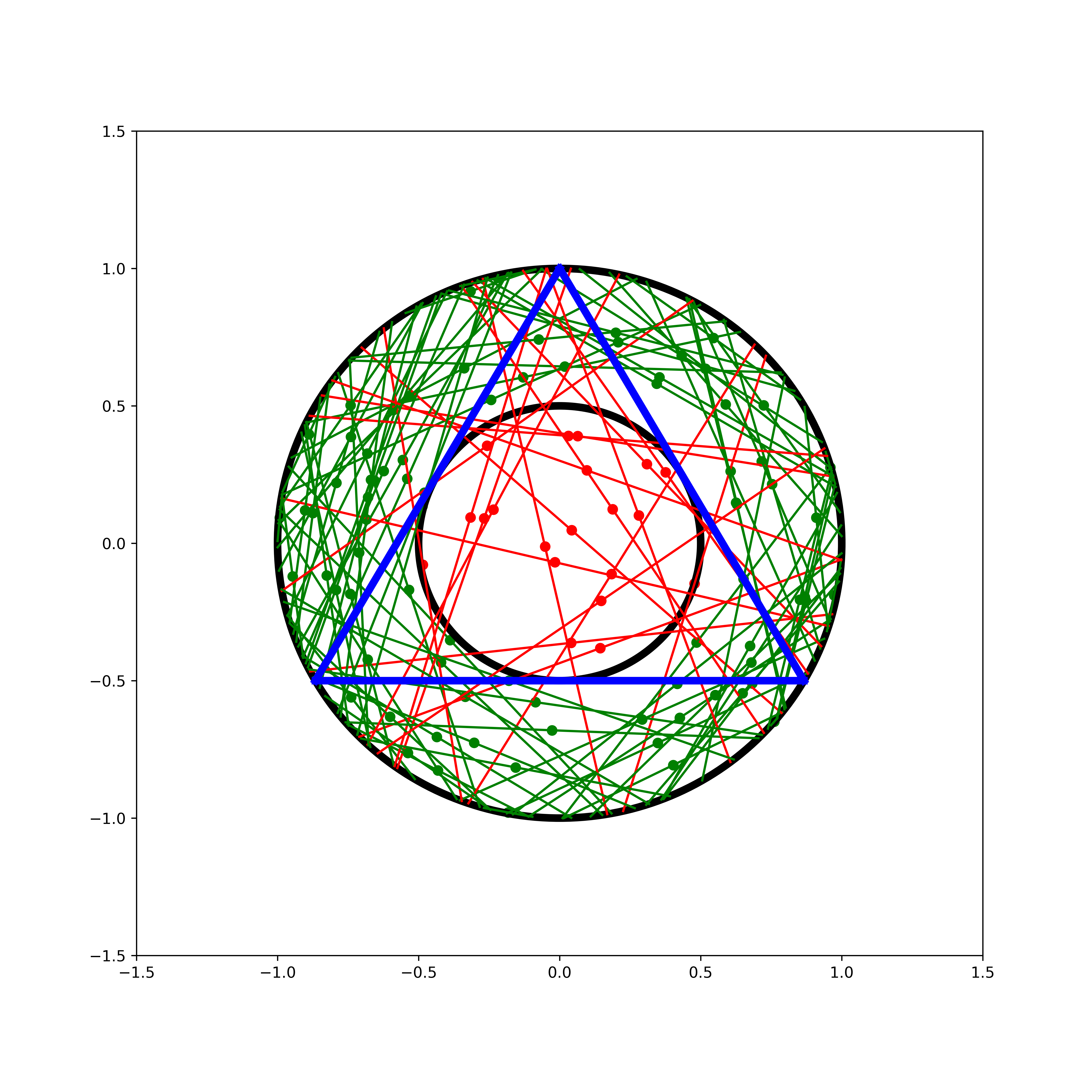
Here I have another circle with radius \(R/2\) to make the result more clear and included the midpoints, showing that the chords are longer than the triangle’s sides when the selected point falls within this circle. Thus the probability approaches \(\frac{1}{4}\) and we have yet another answer!

An Ill-Posed Problem

How do we reconcile these different answers? In the words of Bertrand himself from his 1889 Calcul des probabilités: “Aucune de trois n’est fausse, aucune n’est exacte, la question est malposée.” (“None of these three [solutions] is false, none are correct, the question is ill-posed”)

The key importance of this problem is that it seems to show that specifying something is “randomly selected” is not a specific enough description without also having a description of the particular process that produces the random variable in question. Even in modern times, this problem has received attention. In 1973, Edwin Jaynes argued in his paper “The Well-Posed Problem” for a principle of “maximum ignorance”, claiming that method 2 is the only of the three processes that is both scale and translation invariant, suggesting that the appropriate way to answer the question is including this aspect as part of the problem.

However, even as recently as 2015, papers have been presented that suggest that Jaynes’s “solution” is still not sufficient. See this 2015 paper Failure and Uses of Jaynes’ Principle of Transformation Groups. From my research on the problem, it appears that there is not yet an authoritative resolution to this problem. Code used in this article can be found here.