The Riemann Zeta Function

The Riemann zeta function is a sort of generalization to the Basel problem. We have the (initial) definition that:

\[ \zeta(s) = \sum_{n=1}^\infty \frac{1}{n^s} \]

However, unlike Euler, Riemann considered this function to be complex-valued, where the above series converges when the real part of \(s\) is greater than one. (Riemann found an alternative formula to extend this function to all complex numbers.)

The Riemann zeta function is one of the most studied functions in modern mathematics. The Riemann hypothesis, a statement related to the behavior of zeroes of this function, has remained an open problem since Riemann first posed it in 1859 and is one of the open Millennium Problems that carries a prize of one million dollars from the Clay Mathematics Institute. In this article I will outlay some of the basic properties of the zeta function and summarize some important results.

Euler product formula

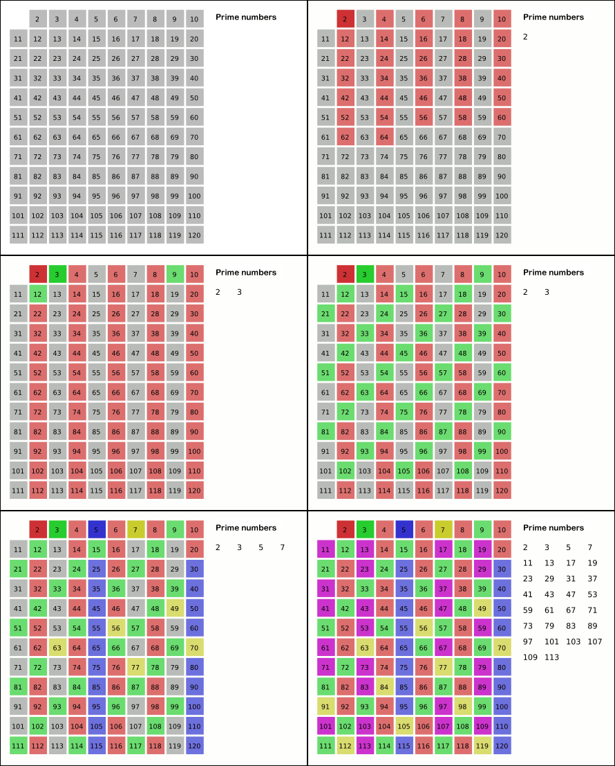
The motivation for considering the zeta function is connected with understanding the distribution of prime numbers. The first such connection was actually discovered by Euler, and is referred to the the Euler product formula. First, it is important that we have an understanding of the Sieve of Eratosthenes, an algorithim used to identify the prime numbers. The idea is simple. First, we eliminate all multiples of 2, then all multiples of 3, and so forth, until we are left with only the prime numbers. The seive is often represented visually as such:

The idea is to use this method to factor the series associated with the zeta function into an infinite product that involves the prime numbers. We begin by looking at the zeta function and terms of the zeta function where the denominator contains a factor of two:

\[\begin{align} \zeta(s) &= 1+\frac{1}{2^s}+\frac{1}{3^s}+\frac{1}{4^s}+\frac{1}{5^s}+ \ldots\\ \frac{1}{2^s}\zeta(s) &= \frac{1}{2^s}+\frac{1}{4^s}+\frac{1}{6^s}+\frac{1}{8^s}+\frac{1}{10^s}+ \ldots \end{align}\]

If we subtract these two expressions, we are essentially “sieving out” all terms with a factor of two:

\[ \left(1-\frac{1}{2^s}\right)\zeta(s) = 1+\frac{1}{3^s}+\frac{1}{5^s}+\frac{1}{7^s}+\frac{1}{9^s}+\frac{1}{11^s}+\frac{1}{13^s}+ \ldots \]

We can repeat this for the next prime number three:

\[ \left(1-\frac{1}{3^s}\right)\left(1-\frac{1}{2^s}\right)\zeta(s) = 1+\frac{1}{5^s}+\frac{1}{7^s}+\frac{1}{11^s}+\frac{1}{13^s}+\frac{1}{17^s}+ \ldots \]

and if we repeat this indefinitely, we will be left with:

\[ \ldots \left(1-\frac{1}{11^s}\right)\left(1-\frac{1}{7^s}\right)\left(1-\frac{1}{5^s}\right)\left(1-\frac{1}{3^s}\right)\left(1-\frac{1}{2^s}\right)\zeta(s) = 1 \]

Rearranging terms this is:

\[ \zeta(s) = \frac{1}{\left(1-\frac{1}{2^s}\right)\left(1-\frac{1}{3^s}\right)\left(1-\frac{1}{5^s}\right)\left(1-\frac{1}{7^s}\right)\left(1-\frac{1}{11^s}\right) \ldots } = \prod_{p \text{ prime}} \frac{1}{1-p^{-s}} \]

This result is perhaps unexpected, but serves to provide certain intuitions regarding the distribution of primes. Firstly, it provides an interesting proof that there is an infinite number of primes as we now have:

\[ \zeta(1) = 1 + \frac{1}{2} + \frac{1}{3} + \frac{1}{5} +\frac{1}{5} +\dots = \frac{2\cdot 3\cdot 5\cdot 7\cdot 11\cdot\ldots}{1\cdot 2\cdot 4\cdot 6\cdot 10\cdot\ldots} \]

and the product can be shown to diverge. (see this page if interested in the details)

More importantly, this formula represents that probability that a given \(s\) integers are all coprime, that is to say that none of these numbers share a common factor. How exactly? First imagine that we want to know the probaility that a single randomly selected number is divisible by 2. This is \(\frac{1}{2}\) since half of the positive integers (\(2, 4, 6, \dots\)) are divisible by 2. Likewise for any another prime number, the probability will be \(\frac{1}{p}\).

If we instead choose \(s\) numbers, we simply multiply these independent probabilities and see that probability of a prime dividing all \(s\) numbers is \(\frac{1}{p^s}\). If I am instead interested in none of the numbers being divisible by this prime \(p\) the probability is the complement \(1-\frac{1}{p^s}\). Finally, if we consider all prime numbers we have:

\[ \prod_{p \text{ prime}} \left(1-\frac{1}{p^s}\right) = \frac{1}{\zeta(s)} \]

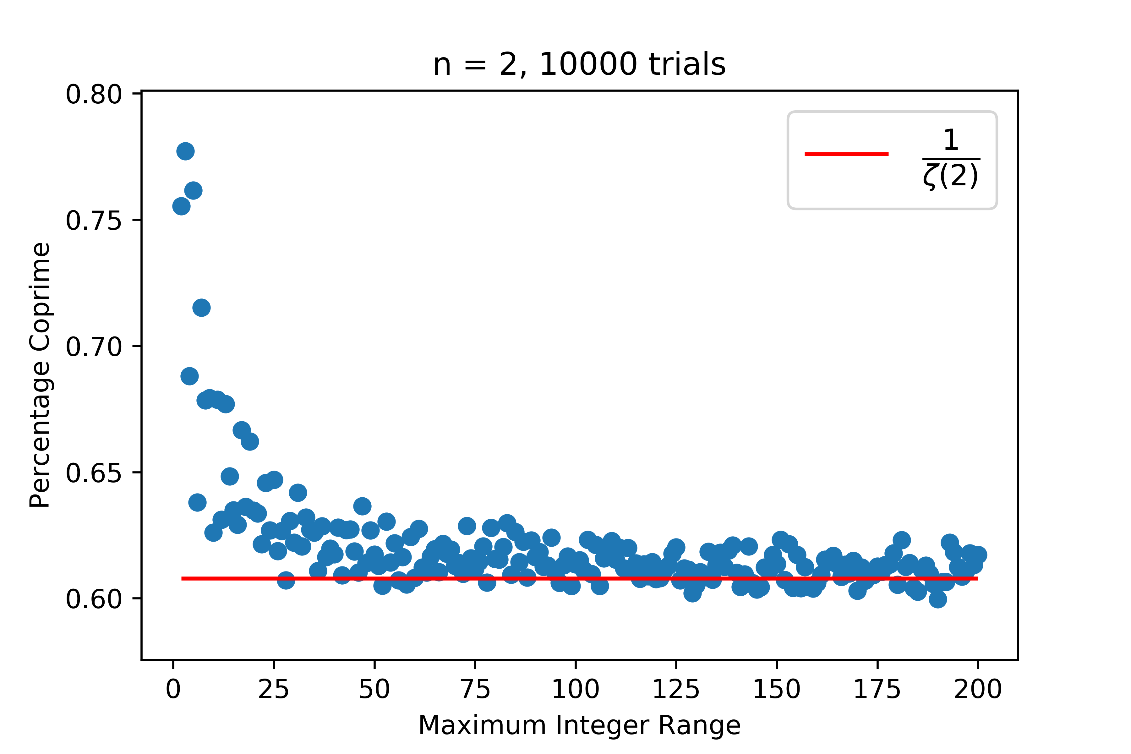
In fact, we can easily write some Python code to select random integers and observe that the probability of selecting two coprime integers approaches \(\frac{1}{\zeta(2)} = \frac{6}{\pi^2}\) as our range of integer selection approaches infinity. Here my code tests selection ranges from (1, 2) to (1, 200), with 10,000 trials for each.

from scipy.special import zeta
from random import randint
from math import gcd, pi
from functools import reduce
import numpy as np

def coprime(n, to):
    l = [randint(1, to) for i in range(n)]
    coprime = int(reduce(gcd, l) == 1)
    return coprime

results = []
max_int = 200
trial_n = 10000

for to in range(2, max_int+1):
    trial = np.mean([coprime(n = 2, to = to) for x in range(trial_n)])
    results.append((to, trial))

Plotting the results, we see that the probability of selecting two coprime integers approaches the expected value of \(\frac{6}{\pi^2} \approx 0.607927\)

import matplotlib.pyplot as plt
%matplotlib inline

plt.scatter(*zip(*results))
plt.title(f"n = 2, {trial_n} trials")
plt.xlabel("Maximum Integer Range")
plt.ylabel("Percentage Coprime")
plt.hlines(y = 1/zeta(2), xmin = 2, xmax=max_int, 
           colors='red', label = r'$\frac{1}{\zeta(2)}$')
plt.legend(prop={'size': 16})
plt.savefig("plot_zeta.png", dpi=600)
plt.show()

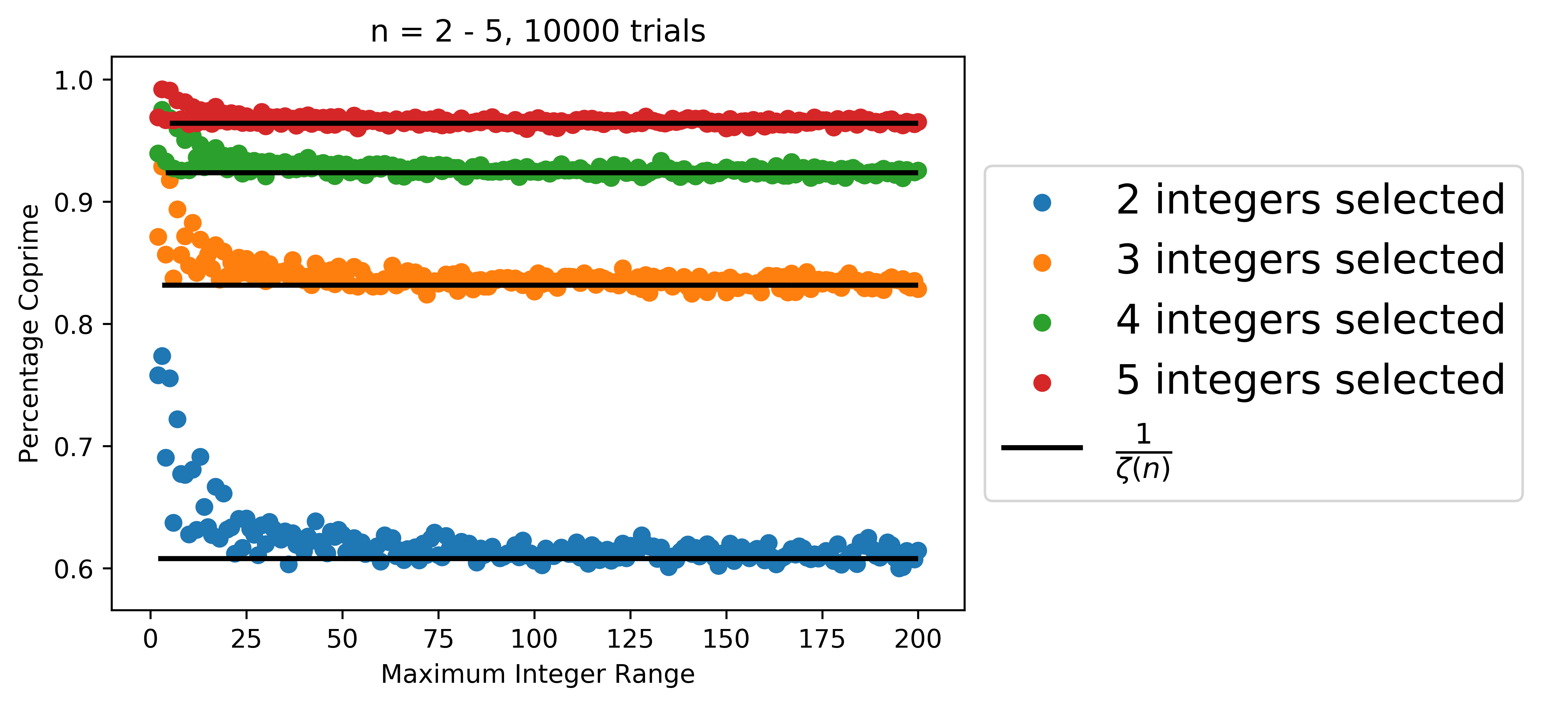
We can repeat the same process for selecting several integers at once:

results = []
max_int = 200
trial_n = 10000

for n in range(2, 6):
    for to in range(2, max_int+1):
        trial = np.mean([coprime(n = n, to = to) for x in range(trial_n)])
        results.append((to, trial, n))

and again plot the results, showing how the limiting behavior agrees with the zeta function:

for n in range(2, 6):
    filt = filter(lambda x: x[2]==n, results)
    x, y, _ = zip(*filt)
    plt.scatter(x, y, label = f"{n} integers selected")

plt.title(f"n = 2 - 5, {trial_n} trials")
plt.xlabel("Maximum Integer Range")
plt.ylabel("Percentage Coprime")
plt.hlines(y = [1/zeta(x) for x in range(2,6)], xmin = range(2,6), xmax=max_int, 
           colors='black', label = r'$\frac{1}{\zeta(n)}$', linewidth=2)
plt.legend(prop={'size': 16}, loc='center left', bbox_to_anchor=(1, 0.5))
plt.savefig("plot_zeta_2.png", dpi=600, bbox_inches='tight')
plt.show()

Note that the preceeding argument would be considered informal. If you’re looking for more background on this problem, check out G. H. Hardy’s An Introduction to the Theory of Numbers where in chapter XVIII (theorem 332) he derives this probability in a much more formal sense.

The Riemann Hypothesis

The brunt of work related to the Riemann zeta function is concerned with the distribution of zeroes of the function. In his 1859 paper On the Number of Primes Less Than a Given Magnitude (original German, English translation) Riemann hypothesized that all zeros of the zeta function are numers with real part \(\frac{1}{2}\), with the exception of the trivial zeros \(-2, -4, -6, \dots\) that had already been previously identified.

Despite overwhelming numerical evidence and much effort for well over a century, a proof of the Riemann hypothesis has yet to be found. Despite this, many conditional proofs exist based upon the Riemann hypothesis and many results exist that relate the zeta function and its zeros to the distribution of prime numbers, despite there not yet being an exact proof of where these zeros exist. I will briefly summarize a few of these results (without proof).

Perhaps most important is the “exact relationship” found by Riemann that describes the number of primes below a given number in relation to the zeros of the zeta function. In particuliar (this is a bit of a doosey, bear with me!) the number of primes less than \(n\) is denoted by \(\pi(n)\) and is given by:

\[ \pi(x) = \operatorname{Ri}(x) - \sum_{\rho}\operatorname{Ri}(x^\rho) \]

where:

\[ \operatorname{Ri}(x) = \sum_{n=1}^{\infty} \frac{\mu(n)}{n} \operatorname{li}(x^\frac{1}{n})\]

or writing things a bit more explicitly:

\[ \pi(x) = \sum_{n=1}^{\infty} \left(\frac{\mu(n)}{n} \int_0^{x^\frac{1}{n}} \frac{dt}{\ln t}\right) + \sum_{\rho} \left(\sum_{n=1}^{\infty} \frac{\mu(n)}{n} \int_{-(\frac{\rho}{n}\ln x)}^{\infty}\frac{e^{-t}}t\,dt)\right) \]

where \(\rho\) is indexed over the zeros of the zeta function, \(\mu(n)\) is the Möbius function, and \(\operatorname{li}(x)\) is the Logarithmic integral function. There seems to be some dispute if this formula has actually been proved in the literature, see this paper and this MathWorld article for more details.

In a closely related yet less obtuse formula, given an upper bound \(\beta\) for the real part of zeros of the zeta function, we have (using Big O notation) that:

\[ \pi(x) - \operatorname{li}(x) = O \left( x^{\beta} \log x \right) \]

Meaning that if the Riemann Hypothesis is true we have:

\[ \pi(x) = \int_0^x \frac{dt}{\ln t} + O\left( \sqrt{x} \log x \right) \]

Conclusion

As we have seen, the Riemann zeta function is inherently linked with the distribution of prime numbers. It actually appears in many other surprising contexts in number theory, as well as physics and statistics. In a future post I will mention a surprising application to divergent series that also appears in quantuum mechanics.

Code used in this article can be found here.