Linear regression is a fundamental aspect of statistics, universally taught in any introductory course. However, what it truly represents and how it functions is often presented in a disjointed way that does not reveal the surprising depth of connections to various mathematical areas, from calculus to sampling distributions.

Here I will begin with the simplest case of simple linear regression and build from the ground up, attempting to create a cohesive look at the intricate mathematics and statistics of regression. I assume that you have a working knowledge of calculus and matrix operations, but review the required statistical tools such as expected value and variance.

Let's start with the simplest of cases. We have two variables: $x$ and $y$.

We would like to find a line that closely matches these points. We will write this equation as:

For now, let's not worry too much about what the "hat" symbol means. It suffices to say that $\widehat{y}$ is the value that lies on our line. How do we find the intercept and coefficient? We will select them to minimize the squared difference between $\widehat{y}$ and $y$. As an equation, where $n$ is our number of data points, we are seeking:

$$ \underset{\beta_0, \beta_1}{\operatorname{arg\,min}} \sum_{i=1}^n (y_i - \widehat{y_i})^2 $$

Note that at this point I've stated no assumptions about normality or anything else we've learned in statistics. We're just finding a line and this is just a calculus problem! A valid question is: "why squared?". The sarcastic answer is because it makes the calculus easier. As we'll see later, this choice is not absolute.

This squared difference goes by many names, such as squared loss, squared residuals, or SSE. To find our solution, we just need a bit of calculus. First a little simplification:

\begin{align} \text{SSE} &= \sum_{i=1}^n (y_i - \widehat{y_i})^2\\ &= \sum_{i=1}^n (y_i - \beta_0 - \beta_1 x_i)^2\\ \end{align}

We take the derivative with respect to $\beta_0$, set equal to zero, and solve to minimize:

The remaining summations are, by definition, sample means of $x$ and $y$. So we have:

Notice that I have added a hat symbol to represent that this is a particular value. Now we can take our derivative with respect to $\beta_1$, substituting the above formula for $\widehat{\beta_0}$:

\begin{align} 0 = \frac{\partial \text{SSE}}{\partial \beta_1} &= \sum_{i=1}^n -2x_i(y_i - \beta_0 - \beta_1 x_i) \\ &= \sum_{i=1}^n -2(x_i y_i - \beta_0 x_i - \beta_1 x_i^2)\\ &= \sum_{i=1}^n (x_i y_i - x_i\bar{y} + \beta_1 x_i\bar{x} - \beta_1 x_i^2)\\ &= \sum_{i=1}^n(x_i y_i - x_i\bar{y}) - \beta_1 \sum_{i=1}^n(x_i^2 - x_i\bar{x})\\ \end{align}

so dividing gives:

Notice again the hat to represent a particuliar solution. A little rearranging gives the following:

$$ \widehat{\beta_1} = \frac{\sum_{i=1}^n(x_i - \bar{x})(y_i - \bar{y})}{ \sum_{i=1}^n(x_i - \bar{x})^2} $$

Just looking at this form, there is something intuitive about it being a measure in the numerator of how often $x$ and $y$ differ from their means at the same time. (More on this in the next section!)

Together, we have a single formula for our line:

\begin{align} \widehat{y_i} &= \widehat{\beta_0} + \widehat{\beta_1}x_i\\ &= \bar{y} - \widehat{\beta_1}\bar{x} + \widehat{\beta_1}x_i\\ &= \bar{y} + \widehat{\beta_1}(x_i - \bar{x})\\ &= \bar{y} + \left(\frac{\sum_{i=1}^n(x_i - \bar{x})(y_i - \bar{y})}{\sum_{i=1}^n(x_i - \bar{x})^2}\right)(x_i - \bar{x}) \end{align}

Above I used the idea of the mean freely, as it is such a common topic. To be precise, given a set $x_1, x_2, \dots, x_n$, we say that the mean is:

In the special case where we know that we have the entire population, as opposed to a sample, we denote this as $\mu$.

The idea of an expected value is closely related. If we have a set of probabilities $p_1, p_2, \dots, p_n$ associated with our data, we say that the expected value is:

which is very intuitively interpreted as a weighted average according to our probabilities. If we have a continuous variable we write:

$$ \operatorname{E}[X] = \int_{\mathbb{R}} x f(x)\, dx $$

where $f(x)$ is our probability density function. This expected value and mean are quite intuitive in that they tell us on average what values our data takes, and have several nice properties, especially that expected value is linear.

If we instead want information about the spread of the data, we will look towards variance, defined as:

$$ \operatorname{Var}(X) = \operatorname{E}\left[(X - \operatorname{E}[X])^2 \right] = \operatorname{E}[X^2] - \operatorname{E}[X]^2 $$

Similarly, the covariance between the two variables is defined as:

$$ \operatorname{Cov}(X, Y) = \operatorname{E}{\big[(X - \operatorname{E}[X])(Y - \operatorname{E}[Y])\big]} = \operatorname{E}[XY] - \operatorname{E}[X]\operatorname{E}[Y] $$

and we can easily see that $\operatorname{Cov}(X, X) = \operatorname{Var}(X)$

The intuition is also easy to see. Just like our regression measured squared residuals, variance measures the squared residuals from the mean of the data to each individual point. Similarly, covariance measures how variance in one variable corresponds to variance in another variable by measuring when they both deviate from their means simultaneously.

The similarity is not just an analogy, as you will see looking at our regression above that

This also makes a sort of intuitive sense, that the slope of the line relating $x$ and $y$ is related to how often they deviate from their means together, relative to how often $x$ deviates from its mean by itself. Again, note the properties that allow us to simplify variances of linear combinations of random variables.

Often you will see this expressed as correlation, which is covariance scaled by variance:

One important distintion to make with the above is that this is the definition for the population variance.

Let's be clear about our definitions of different symbols. Suppose we have a variable $X$. Then the population parameters, taken across every instance of $X$, are:

The population mean, $\mu = \operatorname{E}[X]$
The population variance, $\sigma^2 = \operatorname{Var}(X)$

In reality, we seldom have the entire population at our disposal and must find a suitable value to use as an estimate. We have already seen one such estimate, the sample mean $\bar{x}$. We use the sample mean so frequently that it is almost taken for granted to use this as an estimate of the population mean, but why is this the case? The answer is that the sample mean $\bar{x}$ is an unbiased estimator of $\mu$, in the sense that the expected value of the sample mean is equal to $\mu$.

Suppose that we have $n$ samples, $x_1, x_2, \dots, x_n$, of the variable $X$. Then:

\begin{align} \operatorname{E}[\bar{x}] &= \operatorname{E}\left[\frac{1}{n} \sum_{i=1}^n x_i \right] \\ &= \frac{1}{n}\operatorname{E}\left[ \sum_{i=1}^n x_i \right]\\ &= \frac{1}{n}\sum_{i=1}^n \operatorname{E}[x_i]\\ &= \frac{1}{n}\sum_{i=1}^n \mu\\ &= \mu \end{align}

So what should we use as our sample variance, meant to estimate $\sigma^2$? A natural first thought is to mirror the sample mean and multiply by the term $\frac{1}{n}$. That is to use the estimator:

$$ s_n^2 = \frac{1}{n} \sum_{i=1}^n (x_i - \bar{x})^2 $$

Notice here that these are the squared differences from $\bar{x}$, which we must use since we do not have access to the population mean $\mu$. This aspect is crucial to notice, as it causes this estimate to be biased. Look what happens when we take the expected value of the difference between the population and uncorrected sample variance:

\begin{align} \operatorname{E} \left[ \sigma^2 - s_n^2 \right] &= \operatorname{E}\left[ \frac{1}{n} \sum_{i=1}^n(x_i - \mu)^2 - \frac{1}{n}\sum_{i=1}^n (x_i - \overline{x})^2 \right] \\ &= \operatorname{E}\left[ \frac{1}{n} \sum_{i=1}^n\left((x_i^2 - 2 x_i \mu + \mu^2) - (x_i^2 - 2 x_i \overline{x} + \overline{x}^2)\right) \right] \\ &= \operatorname{E}\left[ \frac{1}{n} \sum_{i=1}^n\left(\mu^2 - \overline{x}^2 + 2 x_i (\overline{x}-\mu) \right) \right] \\ &= \operatorname{E}\left[ \mu^2 - \overline{x}^2 + \frac{1}{n} \sum_{i=1}^n 2 x_i (\overline{x} - \mu) \right] \\ &= \operatorname{E}\left[ \mu^2 - \overline{x}^2 + 2(\overline{x} - \mu) \overline{x} \right] \\ &= \operatorname{E}\left[ \mu^2 - 2 \overline{x} \mu + \overline{x}^2 \right] \\ &= \operatorname{E}\left[ (\overline{x} - \mu)^2 \right] \\ &= \operatorname{Var} (\overline{x}) \\ &= \operatorname{Var}\left( \frac{1}{n} \sum_{i=1}^n x_i \right)\\ &= \frac{1}{n^2}\left( \sum_{i=1}^n \operatorname{Var}(x_i) \right)\\ &= \frac{1}{n^2}\left( n \sigma^2 \right)\\ &= \frac{\sigma^2}{n} \end{align}

So that:

$$ \operatorname{E} \left[ s^2_n \right] = \sigma^2 - \frac{\sigma^2}{n} = \frac{n-1}{n} \sigma^2 $$

From the coefficient, we can see that this sample variance is biased by underestimating the true population variance, especially for a small $n$. The solution is to apply Bessel's correction, where we instead estimate using:

$$ s^2 = \frac{1}{n-1} \sum_{i=1}^n (x_i - \bar{x})^2 $$

As we can see this is now an unbiased estimate, using the above:

Now we're prepared to look at regression of multiple variables. Suppose I am trying to predict $y_i$ as a linear function of $p$ variables $x_{i,1}, x_{i,2}, \dots, x_{i,p}$ My predicted values will be given by:

$$ \widehat{y_i} = \beta_0 + \beta_1 x_{i,1} + \beta_2 x_{i,2} + \dots + \beta_p x_{i,p} $$

A convenient way to represent this is through matrices, which I denote with bolded letters. I will write the following to represent a dataset with $n$ observations:

and our intercept and coefficients as:

Now we can see why we have the extra column of ones in $\textbf{x}$:

Finally, we will write the difference between our actual and fitted values:

Now that we have everything set up, it's time to minimize our squared residuals. Almost just like before, we want to minimize:

But we can now rewrite our squared error as:

simplifying:

Now taking the gradient with respect to $\boldsymbol{\beta}$ and setting equal to 0:

Again I add a hat symbol to represent a particular solution. Let's confirm that this is equivalent to our solution for a single variable. We have:

All together now:

Starting with the coefficient:

That wasn't too painful. Note that at this point, I still haven't done any statistics!! This is purely a calculus problem so far of finding the vector $\widehat{\boldsymbol{\beta}}$ that minimizes our squared errors. Let's finally add some statistics to the mix.

The univariate normal distribution is given by the equation:

where we have mean $\mu$ and variance $\sigma^2$. (You can integrate this function to confirm this fact!).

This distribution is central to statistics for several reasons. Most prominently perhaps is the Central limit theorem that shows that random samples of variables, even if they are not normal themselves, can be described by a normal distribution. Again, the sarcastic answer is that they also make our calculations much easier. In the context of regression, we use the normal distribution as part of our statistical assumptions to infer information that lies outside our observed variables.

Remember that everything that we have done thus far has been completely deterministic, but also limited in a sense. For any arbitrary number of variables $x_1, x_2, \dots, x_p$ and variable $y$, we have found an exact solution to the line that minimizes our squared residuals. But what about the data that we haven't observed? So far we haven't been able to say anything about how accurate we believe our relationship is, or provide any sort of error bounds for future predictions. All that we have is our deterministic $\widehat{\boldsymbol{\beta}}$. Remember that I said that the hat symbolizes that this is an estimate, particularly an estimate determined from our given data. What we would like to do is develop a set of assumptions that allows us to understand the relationship between $\widehat{\boldsymbol{\beta}}$, our estimate, and a theorized $\boldsymbol{\beta}$, the true coefficients that describe the relationship between our variables.

In matrix form we will assume the model:

$$ \textbf{y} = \textbf{x} \boldsymbol{\beta} + \boldsymbol{\epsilon} $$

where $\boldsymbol{\epsilon}$ is a random variable of "noise". (Otherwise, the data would be perfectly linear!).

Note the use of $\boldsymbol{\beta}$ without the hat symbol. This $\boldsymbol{\beta}$ is the vector of "true" coefficients and $\widehat{\boldsymbol{\beta}}$ will be our estimate of these coefficients. We will still calculate $\widehat{\boldsymbol{\beta}}$ in the same way, but now it is a statistical variable rather than a fully deterministic quantity.

Here we will have further requirements on $\boldsymbol{\epsilon}$ that are crucial. Specifically, we assume that $\boldsymbol{\epsilon}$ is given by a normal distribution with a mean of 0 and some constant variance $\sigma^2$.

We also assume that variance and mean is not correlated with $\textbf{x}$. That is for all $[x_{i,1}, \dots, x_{i,p}]^T$:

$$ \operatorname{E}[\boldsymbol{\epsilon} | [x_{i,1}, \dots, x_{i,p}]^T] = 0, \quad \operatorname{Var}[\boldsymbol{\epsilon} | [x_{i,1}, \dots, x_{i,p}]^T] = \sigma^2 $$

Finally, we assume that each $\epsilon$ is independent, that is it has the covariance matrix:

To be precise, we are saying that the errors are a Multivariate normal distribution given by $\boldsymbol{\epsilon} \sim \mathcal{N}(0,\, \sigma^2 I_n)$

What does this all mean intuitively? First, saying that our errors have mean zero means that assume that the model is valid for all values of our independent variable. In real life, we very well could have pockets of values where the "true" coefficients vary between different inputs, especially if there is a variable that we are unable to record.

Our assumption of constant variance rules out possibilities where the spread of our variable $\textbf{y}$ is changing over time. Imagine for instance a machine that slowly deteriorates in performance over time and becomes more sporadic. This would violate the assumption of constant variance, called homoscedasticity.

Lastly, our assumption about independence (the diagonal covariance matrix) is one of the most likely to fail for any situation that includes a time component, as it states that the error associated with each point is not related to those close to it. In all, we must be very careful about these assumptions, and it is a crucial step to empirically measure these values before drawing any further conclusions about our data. However, if we can reasonably assume these pieces, we can say much more about our data and about the nature of our predictions.

Given the assumptions above, there is much that we can say about our predicted values of $\widehat{\boldsymbol{\beta}}$. First, let's rewrite our estimate in terms of the "true" coefficients $\boldsymbol{\beta}$:

\begin{align} \widehat{\boldsymbol{\beta}} &= (\textbf{x}^T\textbf{x})^{-1}\textbf{x}^T\textbf{y}\\ &= (\textbf{x}^T\textbf{x})^{-1}\textbf{x}^T(\textbf{x}\boldsymbol{\beta} + \boldsymbol{\epsilon})\\ &= (\textbf{x}^T\textbf{x})^{-1}\textbf{x}^T\textbf{x}\boldsymbol{\beta} + (\textbf{x}^T\textbf{x})^{-1}\textbf{x}^T\boldsymbol{\epsilon}\\ &= \boldsymbol{\beta} + (\textbf{x}^T\textbf{x})^{-1}\textbf{x}^T\boldsymbol{\epsilon} \end{align}

We can calculate the expected value:

and the variance:

Since we assumed $\boldsymbol{\epsilon}$ to be normal, we see that we have that our predictions themselves are normally distributed! In particular:

There are several interesting things here. First, notice that the expected value of our prediction is the true value of $\boldsymbol{\beta}$, meaning that on average, our predictions will match the true coefficients.

We also have some interesting information from the covariance matrix $\sigma^2 (\textbf{x}^T\textbf{x})^{-1}$, which not only gives us information about how much our predictions will vary, but also shows us the correlation between our predictions of different coefficients, for instance $\operatorname{Cov}(\widehat{\boldsymbol{\beta_0}}, \widehat{\boldsymbol{\beta_1}})$

We can use this normal distribution to make a confidence interval for our prediction of coefficients. Realize however that we don't have $\sigma^2$ or $\boldsymbol{\beta}$, the population parameters. Instead, as discussed in the section on the Bessel correction, we must use the samples that we have for these quantities.

Lastly, we can also find the expected value and covariance matrix for our observed residuals $\boldsymbol{e}$, which you may be surprised at first glance to compare with our theoretical residuals $\boldsymbol{\epsilon}$.

Let $\textbf{H} = \textbf{x} \boldsymbol{\beta} \textbf{y}^T = \textbf{x}(\textbf{x}^T\textbf{x})^{-1}\textbf{x}^T$. The residuals can be rewritten as:

\begin{align} \boldsymbol{e} &= \textbf{y} - \widehat{\textbf{y}} \\ &= \textbf{y} - \textbf{H}\textbf{y} \\ &= ( I_n - \textbf{H})\textbf{y}\\ \end{align}

Take note of the following:

$$(I_n - \textbf{H})^T = (I_n - \textbf{H})$$ $$(I_n - \textbf{H})^2 = (I_n - \textbf{H})$$

So we have:

What's the intuition here? Regression does guarantee that if our assumptions are met, that the expected value of our errors is zero. Interestingly however, the variance of these errors is not just $\sigma^2$, but depends on the data and its covariance as shown above.

Our approach so far seems a little backward. We took a deterministic method, then as almost an afterthought applied a whole slew of assumptions about our data. At no point were we able to incorporate any knowledge about the data itself; what if we had some prior information about $\boldsymbol{\beta}$? We were able to make several deductions, but they very much were consequences of our assumptions applied to our model, which was selected without incorporating any information about these assumptions. Is there a way that we can start from the assumptions alone and derive the model in a probabilistic fashion, not as a minimization problem?

The answer is a resounding yes. What we have seen so far is Ordinary Least Squares regression, but as we will soon see, many variations are derived from tweaks to our assumptions and methods of estimation.

We will begin by first examining two estimation methods, maximum likelihood estimation and maximum-a-posteriori estimation, seeing how they relate to our previous Ordinary Least Squares solution.

Note: For the remainder of the article I have not included intercept terms. This is purely for the sake of simplicity of presentation. To see that the difference is trivial, imagine that instead of including an intercept we have shifted our response variable so that the intercept would pass through the origin, making it unnecessary.

In maximum likelihood estimation, we derive results by considering the probability that our data $\mathcal{D} = \textbf{d}_1, \dots, \textbf{d}_N$ is generated from a given $\boldsymbol{\beta}$, that is:

We define likelihood as the following joint distribution, with the assumption that our samples $\textbf{d}_1, \dots, \textbf{d}_N$ are independent and identically distributed:

We define our MLE estimate as the $\boldsymbol{\beta}$ that maximizes this likelihood. As a practical matter, we usually work with the equivalent log-likelihood:

Now we can derive the MLE estimate of linear regression. We have that each observation comes from the model:

We still assume that:

so that for each individual response:

The probability is:

Now we can find the likelihood for a given $y_1, y_2, \dots, y_N$:

Finally, we can compute the MLE solution:

Miraculously this is the same as ordinary least squares if $\sigma$ is constant! We came to the same solution from a completely different perspective, arriving at our model as a deduction from our assumptions about our errors. As I mentioned, however, this is not the only method of regression. We still haven't been able to incorporate any potential prior knowledge we may have about our coefficients. With the next method, we will be able to accomplish this.

First, we start with Bayes rule, which gives the posterior probability:

here we refer to $P(\boldsymbol{\beta})$ as our prior distribution, $P(\mathcal{D} | \boldsymbol{\beta} )$ is the same likelihood we used above, and $P(\mathcal{D})$ is the probability of our data.

Instead of maximizing just our likelihood, we will maximize the posterior probability and be able to include information about our prior distribution $P(\boldsymbol{\beta})$. We define:

We can see that the only difference between this and MLE is that we have added a term that allows us to augment our likelihood with our prior information about how likely or unlikely a particular set of coefficients is. This allows us to bend our solution to satisfy additional constraints or incorporate information we have seen in the past. With this tool in hand, we will be able to define several new methods of regression.

For our first new method, called ridge regression, we will assume a normal distribution on each of $\boldsymbol{\beta}_1, \dots, \boldsymbol{\beta}_p$ with constant variance $\tau^2$. Calculating the MAP estimate:

writing $\lambda = \frac{\sigma^2}{{\tau^2}}$ we have:

What we see here is that ridge regression has the usual measure of squared residuals but also penalizes large coefficients by adding their squared value, i.e. the $\ell_2$ norm, times some constant $\lambda$ that we must also determine.

I will denote this function as PRSS (penalized residual sum of squares). Taking the derivative with respect to $\boldsymbol{\beta}$ and assuming that we have standardized $\textbf{X}$ and centered $\textbf{y}$:

\begin{align} 0 = \frac{\partial \text{PRSS} (\boldsymbol{\beta})_{\ell_2}}{\partial \boldsymbol{\beta}} &= -2\textbf{X}^T(\textbf{y} - \textbf{X}\widehat{\boldsymbol{\beta}}) + 2\lambda\widehat{\boldsymbol{\beta}}\\ &= \textbf{X}^T\textbf{X}\widehat{\boldsymbol{\beta}} - \textbf{X}^T\textbf{y} + \lambda\widehat{\boldsymbol{\beta}}\\ - \widehat{\boldsymbol{\beta}}(\textbf{X}^T\textbf{X} - \lambda I_p) &= - \textbf{X}^T\textbf{y}\\ \widehat{\boldsymbol{\beta}}_{RIDGE, \lambda} &= (\textbf{X}^T\textbf{X} + \lambda I_p)^{-1}\textbf{X}^T\textbf{y} \end{align}

Firstly, why do we standardize $\textbf{X}$ and center $\textbf{y}$? If we did not do so and have coefficients on very different scales, the value of the penalty term $\lambda \lVert \boldsymbol{\beta} \rVert_2^2 $ is negated.

Look at the similarity to our OLS solution. Setting $\lambda$ equal to 0 is the same as OLS! We have simply added the shrinkage constant $\lambda$ to the diagonal of the matrix $\textbf{X}^T\textbf{X}$, which is related to the covariance of our observed variables.

What is the effect of ridge regression on our predictions? By adding additional information on the prior distribution, we have biased our predicted values away from the true coefficients.

Let $\textbf{R} = \textbf{X}^T\textbf{X}$. We can rewrite the ridge regression prediction:

now taking the expectation:

we can see how far away from an unbiased estimate we have with ridge regression.

We can also rewrite ridge regression as OLS with an augmented data set. Consider:

which is exactly ridge regression! It is interesting to see these relationships between ridge regression and OLS, especially the data augmentation technique that at first glance seems to be concerning from a theoretical standpoint. Regardless, ridge regression is a popular method, where in practice the use of ridge regression (and what $\lambda$ to use) is based upon the performance of our model. Especially in situations where we have a reason to expect coefficients that are very small and normally distributed, this model performs very well.

The derivation of the LASSO regression is nearly identical to ridge regression, but instead of assuming our coefficients are normally distributed, we will suppose that they follow the Laplace distribution with mean 0 and parameter $b$:

Again using the MAP estimate:

again we make a substitution, this time $\lambda = \frac{\sigma^2}{{b}}$ and have:

One major difference is that because of the use of an absolute value, we cannot easily take a derivative to find an analytic solution. We can, however, quantitatively solve and make comparisons with how LASSO shrinks our estimate in comparison to ridge regression. Look at the below visualizations of the norms used in LASSO and ridge respectively:

In ridge regression, while we can arbitrarily shrink our coefficients, none will ever be eliminated. On the other hand, the $\ell_1$ norm's "sharp edge" allows for variables to be removed, allowing LASSO to be used as a sort of heuristic for feature selection. This also matches the intuition of assigning a Laplacian prior distribution, as varying the $b$ parameter causes the distribution to peak more sharply at 0, corresponding to eliminating more variables from consideration.

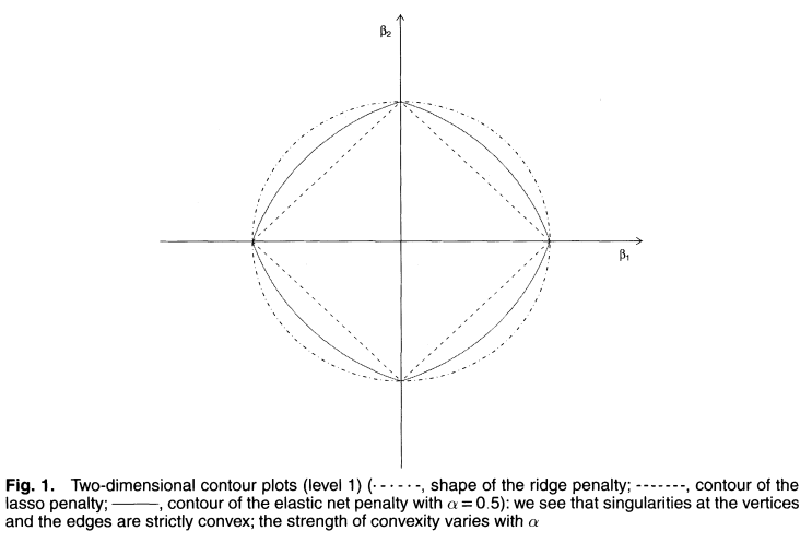
As a final consideration of setting different priors with the MAP estimate of linear regression, we briefly turn our attention to the elastic net. It takes the form:

As can be inferred from the formulation, the elastic net combines the penalty that is given by the LASSO and ridge regressions, as can be visualized by comparing the penalties of the three methods:

For more information, you can read the original paper. There is also a probabilistic interpretation, here are two papers that I have found but not yet had a chance to read.

I've saved the best for last, I promise. The final estimator we will consider is the James-Stein estimator, which presents one of the most interesting paradoxes in statistics.

Suppose for a moment that I take one single sample from a multivariate normal distribution. As I only have a single point, maximum likelihood estimation would tell me that, given my current information, this is the most likely value for the mean of the distribution. We define the risk for such an estimate as the average squared difference between our estimate and the actual value. So if I collect one sample:

the risk would be:

MLE performs rather well in terms of this measurement. We can show that for a scaled normal distribution $\mathbf{X}\ \sim\ \mathcal{N}(\boldsymbol\theta,\, I_n)$ that the expected value of this risk is equal to 1, that is:

This also makes a sort of intuitive sense, in that if we select a single observation as our estimate of a multivariate normal distribution that we would expect the total deviation to remain within roughly one standard deviation of the mean.

Surprisingly in 1961, the statistician Charles Stein and his student Willard James produced a different sort of estimation method that can be shown to have a uniformly lower risk than MLE for three or more dimensions. What takes this from surprising to nearly unbelievable is that this method works by taking the original MLE estimate and shrinking it by a factor that is inversely proportional to the squared norm of our observation. Think about how unintuitive this is for a moment. Even under the supposition that our variables are uncorrelated, the James-Stein estimator uses the entire sample to determine how much to shrink our estimate. They could be completely unrelated quantities like measurements of the speed of light and the price of tea in China, yet this relation would still hold!

Still considering the above case of taking a single sample from the normal distribution $\mathcal{N}(\boldsymbol\theta,\, I_n)$ the James-Stein estimator is the following:

$$ \boldsymbol{\hat\theta_\text{JS}} = \left(1 - \dfrac{p-2}{\lVert\mathbf{x}\rVert^2}\right)\mathbf{x} $$

For instance, suppose we had sampled $\textbf{x} = \boldsymbol{\hat\theta}_\text{MLE} = (-0.8859395, 0.2597109, -1.1817573)$. Our shrinkage factor would be:

$$ \left( 1 - \dfrac{1}{-0.8859395^2 + 0.2597109^2 + -1.1817573^2}\right) = .555336 $$

giving:

$$ \boldsymbol{\hat\theta_\text{JS}}^T = .555336\begin{bmatrix}-0.8859395\\ 0.2597109\\ -1.1817573\end{bmatrix} = \begin{bmatrix} -0.4919941 \\ 0.1442268 \\ -0.6562724 \end{bmatrix} $$

With a good bit of statistical work, we can quantify how much better the James-Stein estimator performs than MLE. Unlike MLE, the risk is not a constant value but depends on several factors such as the number of variables (adding more decreases risk) and how close the mean vector is to zero. To be exact, the risk for the James-Stein estimator is:

$$ \text{Risk}_\text{JS} = 1 - \dfrac{(p-2)^2}{p}\operatorname{E}\left[\dfrac{1}{\mathbf{\lVert x \rVert}^2}\right] $$

To apply this to regression, we use the following variant of the James-Stein estimator:

$$ \widehat{\boldsymbol{\beta}}_{JS} = \widehat{\boldsymbol{\beta}}_{OLS}\left( 1 - \frac{(p-2)\frac{\sigma^2}{n}}{(\widehat{\boldsymbol{\beta}}_{OLS} - \tilde{\boldsymbol{\beta}})^T(\widehat{\boldsymbol{\beta}}_{OLS} - \tilde{\boldsymbol{\beta}})} \right) $$

where $\sigma^2$ is the variance of our residuals and $\tilde{\boldsymbol{\beta}}$ is our vector of coefficients that we have selected to shrink towards, much in a similiar fashion as the LASSO and ridge estimators. For more information, take a look at this simulation that I made in R and see this paper for details about how the James-Stein estimator for regression performs.

As we have seen in this article, the topic of regression, which at first glance appears to be rather simple, has a diversity of subtleties and nuance. This is just a small yet representative sample (pun intended) of the sort of statistics that can be done in estimating models.

Keep in mind that this is just linear regression, we didn't even touch any other types of models. Especially when reasoning under statistical uncertainty or dealing with problems such as causality, heteroscedasticity, or other more advanced topics, a solid understanding of these fundamentals that underpin linear regression is a powerful tool.

If you have any questions or think you may have spotted an error in my calculations, please do not hesitate to contact me!

Simple linear regression
Simple Linear Regression in Matrix Format
Parameter Estimation in Probabilistic Models, Linear Regression and Logistic Regression
A Probabilistic Interpretation of Regularization
Regularization: Ridge Regression and the LASSO
Improving Efficiency by Shrinkage, The James-Stein and Ridge Regression Estimators